Wind pressure characteristics of chinese traditional timber buildings through wind tunnel tests

Mean wind pressure characteristics

The mean wind pressure coefficients \({C}_{p,\mathrm{mean}}\) distributed on the upper and lower surfaces of the roofs of five building models are presented in Fig. 9. As shown in Fig. 9a, under the perpendicular and oblique wind directions (0° and 90°), the mean pressure coefficient is negative at the leading edge of the windward side of the roof, and the maximum negative pressure coefficient is −0.2, while it gradually increases into positive wind pressure near the main ridge with the maximum positive pressure coefficient of 0.3. The crosswind and leeward sides predominantly show negative pressures, with the largest value of −1.2 occurring near sloping ridges. Notably, the lower eave surface demonstrates higher positive pressures than the upper windward surface, while maintaining similar negative pressure magnitudes to the upper crosswind side. The maximum positive pressure coefficient (0.4) occurs at roof pediments under perpendicular winds.

a Model-0, b Model-1, c Model-2, d Model-3, e Model-4-Main roof, f Model-4-Outer eave.

Comparing the smooth-surfaced Model-0 and tiled Model-2, both featuring hip-and-gable roofs, reveals that geometric details significantly influence pressure distributions. While both models show similar distribution patterns, Model-2 exhibits reduced pressure amplitudes. Model-0 demonstrates steeper negative pressure gradients on crosswind sides, particularly at 0° and 90° winds, and higher pediment pressures (0.4 vs 0.3 in Model-2), suggesting that traditional ornaments serve both esthetic and aerodynamic purposes by mitigating wind pressures. Analysis of Model-1 and Model-2 demonstrates that roof type affects pressure distribution primarily at ridge junctions during oblique winds. Model-2 develops localized high pressures at hanging/sloping ridge junctions, while Model-1’s simpler geometry results in smaller frontal areas and more uniform pressures. The comparison between the flat corner Model-2 and the upturned corner Model-3 indicates that the upturned corners have a higher pressure gradient, especially on the crosswind side. The double-eave Model-4 shows increased leading-edge negative pressures but reduced windward positive pressures compared to the single-eave Model-3, and the outer eave exhibits significantly elevated positive pressure coefficients on the windward upper surface.

The mean pressure distribution characteristics on the roof surfaces of five building models are qualitatively discussed above. Here, the coefficients are quantitatively analyzed by partitioning the roof into small subareas, then extracting and averaging the pressure coefficients within each subarea. Due to the symmetry of the building geometries, the measured data of a quarter roof surface under all wind directions is used here. The quarter roof is partitioned into ten subareas. Figure 10a, b demonstrates the roof partitioning schemes on the upper and lower surfaces of the roof for five building models, respectively.

a Roof area partitioning (Subareas I~Vl) of the upper surface, b Roof area partitioning (Subareas VI~X) of the lower surface.

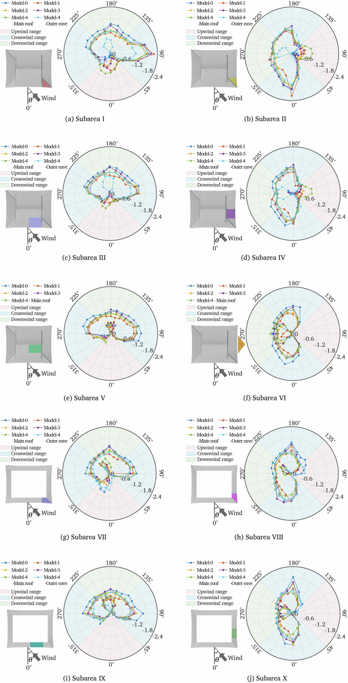
The rose plots in Fig. 11a–j display the area-averaged pressure coefficients for Model-0 to Model-4 across Subareas I to X under all wind directions. The radial coordinates in these plots are negative, with values ranging from 0 to −1.5, while the small ring-like polylines near the center, plotted in reverse, represent positive coefficients. In general, the coefficient polylines form elongated ovals, with their major axes aligned with the crosswind direction and minor axes along the windward or leeward direction. Comparing subareas horizontally—such as those on the building width side versus their counterparts on the depth side—reveals that along the minor axis, the area-averaged pressure coefficients reach local maxima for Subareas I, III, V, VII, and IX (180°) but local minima for Subareas II, IV, VI, VIII, and X (270°). Nearly all polylines attain their most negative peak values along the major (crosswind) axis. On the upper roof surface, peak negative coefficients are comparable for corresponding subareas on both sides (e.g., Subarea I vs. II), whereas on the lower surface, the width-side subareas (VII and IX) exhibit smaller peaks than those on the depth side (VIII and X). A vertical comparison of subareas on the same roof side shows that corner subareas (I and II) on the upper surface experience larger negative coefficients than other subareas (III–VI), while on the lower surface, corner subareas (VII and VIII) demonstrate smaller-magnitude coefficients compared to non-corner subareas (IX and X). Next, a comparative analysis of area-averaged pressure coefficients across different models will be presented. The plotted values are predominantly negative, with peak negative coefficients ranging from −0.5 to −1.5, though some upwind subareas exhibit positive values not exceeding 0.5. In general, negative pressure coefficients of all models are as follows: the smooth-surfaced model (Model-0) exhibits the highest magnitudes, followed by the upturned-corner gable-and-hip roof model (Model-3). The double-eave model (Model-4) shows comparable or slightly higher values at its outer eave than at its main roof, both exceeding those of the flat-corner gable-and-hip roof model (Model-2). The standard hip roof model (Model-1) consistently yields the lowest negative coefficients.

a Subarea I, b Subarea II, c Subarea III, d Subarea IV, e Subarea V, f Subarea VI, g Subarea VII, h Subarea VIII, i Subarea IX, j Subarea X.

To investigate the effects of geometric details on wind pressure, a comparison is made between the results of Model-0 and Model-2. With the exception of certain localized upwind conditions, the polyline patterns of area-averaged pressure coefficients for Model-0 and Model-2 exhibit identical shapes, though Model-0 demonstrates approximately 1.34 times greater amplitude on average. The presence of roof tiles on the upper surface and rafters on the lower surface appears to mitigate wind pressure effects, as previously observed in pressure contour plots. Notably, within specific oblique upwind directions (315°–360° for subareas I, III, V and 90°–135° for subareas II, IV), the tiled roof (Model-2) exhibits relatively larger negative pressure coefficients. This phenomenon occurs because the smooth roof (Model-0) develops localized positive pressure near the sloping ridge, partially offsetting the negative pressure.

Model-1 and Model-2 are compared to examine how roof type (with a specific focus on hip roofs versus gable-and-hip roofs) affects wind pressure. When comparing the hip roof with the gable-and-hip roof, both featuring flat roof corners but differing in overall form, the hip roof generally shows slightly reduced negative pressure coefficients across most wind directions. The most significant differences occur in downwind conditions for width-side subareas (I, III, V, VII, IX) and crosswind conditions for depth-side subareas (II, IV, VI, VIII, X), where the gable-and-hip roof’s negative pressure coefficients reach up to 1.28 times greater than those of the hip roof. As illustrated in Fig. 9a, b, under perpendicular crosswinds (90° for Subarea I and 0° for Subarea II), the hip roof corners develop the most extreme negative pressures among all models, reaching a coefficient of −1.49.

The impact of a flat or upturned roof corner on wind pressure is explored by comparing Model-2 and Model-3. Analysis of the flat-corner versus upturned-corner configurations reveals that the upturned design consistently generates greater negative pressures on all width-side subareas during downwind conditions (most pronounced at 180° for subareas I, III, V, VII, IX). Similar enhancement occurs on opposite roof-side subareas under crosswind conditions (peaking at 0° and 180° for subareas II, IV, VI, VIII, X). These findings indicate that corner form primarily influences pressure distributions when winds approach perpendicular to the building width, with upturned corners amplifying negative pressure effects.

To study the effects of double eaves on wind pressure, a comparison is conducted between Model-3 and Model-4. The double-eave configuration demonstrates two key effects relative to the single-eave roof: moderate reduction of negative pressure on the main roof’s upper surface coupled with increased negative pressure on its lower surface. The outer eave maintains comparable negative pressure levels during crosswind and downwind conditions. Conversely, under upwind conditions, all subareas exhibit positive pressure coefficients, particularly pronounced on the outer eave’s upper surface.

Fluctuating wind pressure characteristics

The contour plots of the fluctuating pressure coefficients under the wind direction 0°, 30°, 60°, and 90° on the upper and lower surfaces of the roofs for the five building models are presented in Fig. 12a–f, respectively. For single-eave models, Model-0, Model-1, Model-2, and Model-3, wind direction 0°, the fluctuating pressure coefficients of the leading edge of the windward roof are relatively larger, then decrease at the windward roof center, and then increase at the main ridge. The upper and lower surfaces of roof corners behind the sloping ridge on the crosswind side take the maximum fluctuating pressure with values of 0.33, 0.39, 0.29, and 0.34 for Model-0, Model-1, Model-2, and Model-3, respectively. The fluctuating degree in the side wind area of Model-3 is relatively high. For the wind direction 90°, the fluctuating pressures of the four models have the same distribution trend as that for wind direction 0°, and comparable maximum values as well. As for the oblique wind directions, 30° and 60°, the largest fluctuating pressure coefficients take place at the windward roof corners and areas behind the hanging and sloping ridges with maximum values of 0.23, 0.17, 0.18, and 0.17, respectively, for the four models, which are obviously smaller compared with those under perpendicular wind directions. However, the fluctuating pressure coefficient distribution on the roof of the double-eave model, Model-4, is different from the other models. Its maximum fluctuating pressure emerges at the windward roof center, with the values of 0.21 for 0° and 0.29 for 90°, while the pressure on the crosswind side fluctuates not so strongly as that on the windward side. The fluctuating pressure coefficient distributions and values are about the same as the other four models.

a Model-0, b Model-1, c Model-2, d Model-3, e Model-4-Main roof, f Model-4-Outer eave.

Non-Gaussian characteristics of wind pressure

The non-Gaussian characteristics of wind pressure are investigated based on the test data of Model-0 smooth-surfaced building. Figure 13 presents the time-history curves and probability density histograms of wind pressure at typical measurement points on the roof of a smooth-surface building. The results demonstrate that the windward leading edge and side-wing corners of the roof are located within the flow separation zone, exhibiting pronounced asymmetry in their wind pressure time–history curves. These regions are characterized by intermittent pulse signals and experience significant wind suction forces. Analysis of wind pressure coefficient probability distributions across additional representative points reveals that, except for localized areas on the windward side, most measurement locations on the smooth-surface roof display distinctly non-Gaussian characteristics in their wind pressure signal distributions.

Time-history curves of Cp and probability density histograms at typical points on Model-0.

Figure 14 shows the distribution of skewness and kurtosis values for all measurement points across five test models. The visualization clearly demonstrates the degree of non-Gaussian behavior in surface wind pressure probability densities. Among these, Model-3 (hip-and-gable roof with upturned eave corners) exhibits the strongest non-Gaussian characteristics, with maximum kurtosis reaching 19.2 and maximum skewness of −2.7. Comparative analysis with Model-2 (hip-and-gable roof with gentle eave corners) confirms that upturned eave corners effectively enhance the non-Gaussian nature of roof wind pressures. This phenomenon occurs as the incoming flow generates vortices of specific dimensions and structures after passing the upturned corners. In contrast, Model-4 (double-eave hip-and-gable roof) shows the weakest non-Gaussian behavior, suggesting that the presence of secondary eaves in multi-tiered roofs disrupts and diminishes the formation of large-scale structural vortices.

a Model-0, b Model-1, c Model-2, d Model-3, e Model-4.

Wind pressure probability density distributions from five representative measurement points with varying kurtosis and skewness values were selected and compared with their corresponding probability density curves fitted using the HPM method, as shown in Fig. 15. The results demonstrate that the HPM-fitted probability density functions show good agreement with the target values for both: (1) weakly non-Gaussian wind pressure cases (Fig. d and e), and (2) strongly non-Gaussian wind pressure cases (Fig. a–c). This confirms that the peak wind pressure values calculated using the HPM yield satisfactory results.

a Point 151, b Point 23, c Point 8, d Point 1, e Point 112.

Peak wind pressure characteristics

Figure 16 presents the distribution of peak wind pressure coefficients on the roofs of the five building models, which are calculated using the HPM translation method. When compared with the mean pressure distribution shown in Fig. 9, it can be observed that the distribution patterns and variation trends of the peak wind pressure are generally consistent with those of the mean wind pressure. Therefore, no further elaboration will be made here. However, it should be noted that the magnitudes and gradients of the peak wind pressure coefficient are significantly greater than those of the mean wind pressure coefficient. For all building models, the maximum negative peak pressure consistently occurs at the crosswind side of the roof corners under perpendicular wind directions, with the peak wind pressure coefficients ranging from −2.2 to −2.5. On the other hand, the maximum positive peak pressure is always found at the roof pediments, with values ranging between 0.8 and 1.2.

a Model-0, b Model-1, c Model-2, d Model-3, e Model-4-Main roof, f Model-4-Outer eave.

The peak wind pressure coefficients are averaged within the ten subareas defined in Fig. 10, yielding the area-averaged peak pressure coefficients of all building models shown in Fig. 17. These results exhibit essentially identical patterns to the area-averaged mean wind pressure coefficient rose diagrams (Fig. 11). For all five building models, the maximum values of area-averaged peak wind pressure consistently occur under perpendicular wind directions, specifically along the 0°–180° and 90°–270° axes in the figure, demonstrating that perpendicular wind directions represent relatively critical wind directions for traditional architecture. The subareas with maximum negative peak pressure are located at the crosswind side of the roof corner (Subareas I and II) under perpendicular wind directions. The highest negative peak pressure coefficient reaches approximately −2.3, observed in Model-1 with the hip roof, followed by Model-0 (smooth surface), Model-3 (upturned-eave hip-and-gable roof), Model-2 (flat-eave hip-and-gable roof), and Model-4 (double-eave hip-and-gable roof), with the minimum value occurring at the outer eave of Model-4. The area with the maximum positive peak pressure is the pediment area (Subarea VI) when facing the wind. However, the magnitude of these positive coefficients is significantly smaller compared to the negative peak coefficient values, with all subareas exhibiting maximum positive pressure coefficients ranging between 0.6 and 1.2.

a Subarea I, b Subarea II, c Subarea III, d Subarea IV, e Subarea V, f Subarea VI, g Subarea VII, h Subarea VIII, i Subarea IX, j Subarea X.

The peak pressure values under a single wind direction, as discussed above, focus on identifying which parts of the building exhibit local peak pressure when subjected to wind from a specific direction. Their significance lies in identifying the optimal or most unfavorable wind directions for the building. In contrast, the all-directional peak pressure, i.e., the peak wind pressure under all wind directions, reflects the ultimate wind pressure state of the building surface when exposed to wind from all possible directions. It aims to provide the most conservative and safest basis for determining peak wind loads in the wind resistance calculation of traditional buildings. All-directional peak pressure coefficients for subareas of all building models are presented in Fig. 18. All roof corners are subjected to maximum wind suction, among which the hip roof and the upturned-corner gable-and-hip roof exhibit the highest wind suction with the pressure coefficients around 2.0–2.2. This is followed by the smooth building and the flat-corner gable-and-hip roof with the pressure coefficients around 1.8–1.9, then by the roof corners of the main roof of the double-eave building with the pressure coefficients around 1.7–1.8, while the lowest wind suction is observed at the outer eave corners of the double-eave building with the pressure coefficients around 1.3–1.6. The wind suction at the roof center part is smaller than that at the corners. Overall, the wind suction on the upper roof surface is consistently greater than that on the corresponding lower roof surface.

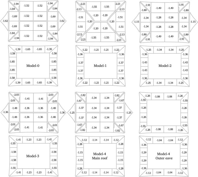
All-directional peak pressure coefficients for subareas of all building models.