
Building morphologies of the USA structures database; a gauntlet feature set

The earliest iterations of Gauntlet utilized ancillary data to create additional features. Ancillary data in this sense is any additional datasets other than the building polygon dataset. These ancillary datasets were, for example, the National Land Cover Database (NLCD)11 and a licensed road network dataset. The NLCD value was assigned to the polygon as a categorical attribute according to the polygon centroid. Another early feature was the measure to the nearest road from the polygon’s closest edge. Collectively these features were grouped as ancillary features.
Issues began to arise as the imagery used to extract the building geometries was much more recent than these ancillary datasets or beyond their coverage. Gauntlet needed to be able to generate morphologies on any polygon dataset regardless of location and availability of current supporting datasets. Because of this need for flexibility, these features generated from ancillary datasets were dropped. The ancillary feature category was retired and replaced by the contextual category of features. This change in feature categories represents the Gauntlet feature set version 1.0 from 2020. Since then, there has been a significant increase in features in the contextual category. This paper describes the Gauntlet version 2.0 feature set developed in 2023. The features we selected for inclusion in this dataset are the features we have found to be informative features through published literature2,3,4,5,6,7. Furthermore, these features function well on a variety of building polygon data sources which span the world without the need for ancillary data and can be computed within reasonable amount of time. Figure 1 shows the overall processing steps for creation for this Gauntlet feature set. The details of each step are described in the Overall Workflow subsection of this Methods section.

The overall workflow for the USA Structures derived Gauntlet dataset.
Preprocessing
The source building data for this Gauntlet feature set is USA Structures12. USA Structures was chosen because of its rich attribution that could be used for potential training labels. USA Structures is divided by state. Each state is stored within its own file geodatabase (file GDB) as a feature class. We use a spatially enabled Postgres database with the PostGIS extension to store the original geometries and attributes from the source.
As feature classes from each file geodatabase were ingested into the central postgres database two preprocessing steps were conducted. First, the geometries were evaluated for the appropriate Universal Transversal Mercator (UTM) zone projection. Secondly, Square Meters (sqmeters), Square Feet (sqft), Latitude (lat), and Longitude (lon) were calculated based off the identified UTM zone projection and stored in the database with the geometries maintaining their original projections. The building dataset has no projection and the original datum is World Geodetic System (WGS) 84.
Features Categories
The 65 features that Gauntlet generates fall within three categories: Geometric, Engineered, or Contextual. Geometric features are simple measures of geometry that describes a physical characteristic of the geometry. Engineered uses two or more geometric features to describe more complex measures of geometry like compactness or complexity. Lastly, the contextual features describe the geometry and its relationship to neighboring geometries within a set distance. Contextual features attempt to replace the need for calculating features using ancillary datasets. This provides a benefit for scaling workflows without the concern of completeness or coverage of other datasets. Contextual features are calculated on multiple scales as inspired by the work of Milojevic-Dupont’s work using urban form to predict building heights13. Many of contextual features are derived using spatial point pattern analysis14,15 and have been studied in earlier works16. Table 2 provides a brief description of the current Gauntlet features. Figure 2 shows a sample of USA Structures symbolized by four different morphology features calculated within the Gauntlet feature set.

USA Structures symbolized by four different Gauntlet features: (Top) complexity_ratio, ipq, (Bottom) n_count_250, and n_size_cv_50.
Geometric Features
Geometric features are the simplest and derived from the direct measurement of a physical property of the geometry. Three of these are features of the geometry’s area in different units: sqft, sqmeters, Shape Area (shape_area). There is one measure of perimeter length: Shape Length (shape_length). Vertex Count (vertex_count) is a count of all the vertices in the geometry. The last feature in the geometric category is Geometry Count (geom_count) which is a count of the number of polygons used to create the shape of the geometry. Most geometries of USA Structures will only have one polygon, occasionally a geometry might have a hole like a courtyard. This hole is represented by a second inner polygon, and the geom_count would be two for this example geometry.
Engineered Features
The next category is engineered. Engineered features are typically derived from one or more geometric features. Among many possible engineered features in the literature, we selected the following for inclusion into the Gauntlet feature set, as we found them to be useful for various classification tasks2,3,4,5,6,7. Complexity Ratio (complexity_ratio) was first introduced by Ritter in the year 182217,18 and is the ratio of Perimeter (shape_length) to the Area (shape_area).
$$complexity\,\_ratio=\frac{shape\_length}{shape\_\,area}$$
(1)
complexity_ratio is a measure that is biased toward smaller geometries, as geometries with smaller areas will have higher complexity ratios. Even geometries with a set shape like a square or equilateral triangle but different areas will have differing complexity ratios. Osserman in 1978 proposed the Isoperimetric Quotient (ipq)19 which is considered more effective measure of compactness than the complexity_ratio18. Despite the multitude of compactness measures proposed20, Osserman’s measure was used for its simplicity and low computational expense. ipq is calculated in the following manner using the earlier described geometric features:
$$ipq=\frac{4\ast \pi \ast shape\,\_area}{shape\_\,lengt{h}^{2}}$$
(2)
ipq, also known as Circularity21, is a true ratio, the possible values are 0 to 1. ipq value of 1 is a perfect circle. Shapes with low ipq values do not maximize their area for the given perimeter. An annulus with a large inner ring is a good example of a low ipq shape. Some fixed shapes like squares and equilateral triangles have a fixed ipq score regardless of their size or orientation, 0.785 and 0.6046 respectively. Figure 3 and Table 3 demonstrate the complexity_ratio and ipq relationship using two different sized equilateral triangles. Figure 4 shows ipq and complexity_ratio values for various geometries.
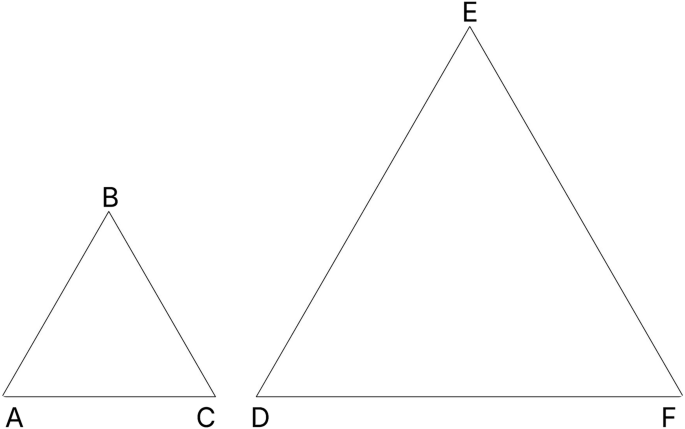
ΔABC and ΔDEF are equilateral triangles. ΔDEF has double the shape_length of ΔABC. ΔABC has double the complexity_ratio of ΔDEF, but they both have the same ipq score: 0.6046. Table 3 provides more details of ΔABC and ΔDEF.

On the left, five examples of ipq values for differently shaped polygons are provided. On the right, the corresponding complexity_ratio values. Note complexity_ratio values are roughly inverted to ipq, while ipq ranges from 0 to 1.
Another engineered feature used is the Inverse Average Segment Length (iasl). This feature is calculated in the following manner:
$$iasl=\frac{vertex\,\_count}{shape\_\,length}$$
(3)
Complexity Per Segment (complexity_ps) describes how much of the overall geometry’s complexity is described within each segment of the geometry. This engineered feature is calculated in the following manner:
$$complexity\,\_ps=\frac{\frac{shape\_length}{shape\_area}}{vertex\_\,count}$$
(4)
Vertices per area (vpa) is another feature that describes the overall complexity of the geometry’s shape. vpa is calculated in the following manner:
$$vpa=\frac{vertex\,\_count}{shape\_\,area}$$
(5)
Envelope Area (envel_area) is the area of the bounding box of a geometry. Longitude Difference (long_dif) is the longitudinal maximum of the geometry subtracted from the longitudinal minimum, while Latitude Difference (lat_dif) is the latitudinal maximum subtracted from the latitudinal minimum. These three features are calculated in a series of computations described in equations 6–13 where x is longitude and y is the latitude of point i.
$$Geom=\{({x}_{i},{y}_{i})| i=1,\ldots ,n\}$$
(6)
$$a=max({x}_{i},\ldots ,{x}_{n})$$
(7)
$$b=min({x}_{i},\ldots ,{x}_{n})$$
(8)
$$c=max({y}_{i},\ldots ,{y}_{n})$$
(9)
$$d=min({y}_{i},\ldots ,{y}_{n})$$
(10)
$$envel\,\_area=long\_dif\ast lat\_\,dif$$
(13)
Contextual Features
Contextual features provide information about how a building geometry relates to its neighbors. The neighbors of a building geometry are all the building geometries whose centroids are within a specific distance. This radius will be referred to as a scan window. Once the neighbors are identified a series of measurements are calculated with the scan window centered on the building geometry being evaluated. The process is repeated with larger scan windows to provide various levels of spatial context. The scan window radii are in 50 m, 100 m, 250 m, 500 m, and 1000 m.
Gauntlet generates two sets of contextual features. The first set being point pattern features, which describe the spatial relationships of all building centroids within the scan window. The second are scale related features, which describe the building areas within the scan window. Many of these features, but not all, have been discussed in previous work16,21 and shown to be successful in classification problems3,4,15,22.
Point Pattern Features
There are two foundational measures which we use to compute many contextual features. The first is Neighborhood Count (n_count) which is the count of all the building centroids within the scan window. To quickly identify the neighbors within the specific distance, we use a cKDtree from scipy23 which was originally proposed by Maneewongvatana and Mount24. The KDtree is a performant spatial index for querying point geometries (centroids) within specific radii. Once the total number of centroids are known within the radius we can then compute the second foundational measure: Nearest Neighbor Distance (nnd). nnd is the measured distance from one centroid of a building’s geometry the nearest neighboring building’s centroid. These two features are used to derive more sophisticated contextual features25.
Observed Mean Distance (omd) is the sum of the nearest neighbor distances of all centroids within the scan window divided by the n_count of the same scan window25. The equation is as follows where di is the nearest neighbor distance between coordinate pair i:
$$omd=\frac{\sum {d}_{i}}{n\_count}$$
(14)
Expected Mean Distance (emd) is the average distance of all centroid neighbor pairs if the centroids were at complete spatial randomness within the scan window25. Expected mean distance is calculated as follows where r is the radius of the scan window:
$$\rho =\frac{\pi \ast {r}^{2}}{n\_count}$$
(15)
$$emd=\frac{1}{2\ast \sqrt{\rho }}$$
(16)
Nearest Neighbor Index (nni) uses omd and emd to describe the overall spatial pattern of points within the scan window. This index has a range of 0 to 2.149125. 0 represents a clustered pattern within the scan window. This could indicate one tightly packed cluster or multiple clusters. 1 represents a random distribution of points within the scan window, e.g complete spatial randomness. 2 or higher represents a pattern close to even dispersion within the scan window where all distances are close to equal25. The full formula for nni is as follows where again di is the nearest neighbor distance between coordinate pair i:
$$nni=\frac{\frac{\sum {d}_{i}}{n\_count}}{0.5\ast \sqrt{\rho }}$$
(17)
Scan Window Intensity (intensity) measures the amount of nni is occurring within the scan window. For example, if two scan windows have the same nni of 0.05, both are highly clustered. However, if one of the windows has a higher intensity that would indicate more clusters or more members in the clusters of one scan window over the other. intensity is calculated with distances from the sample point, i.e. center of the scan window, to each individual point in the scan window14. We utilized the KDtree again to compute this metric. Figure 5 displays nni and intensity values calculated at 100m buffers on four different scenarios. The formula for intensity is as follows where \({d}_{i}^{2}\) is the squared distance of each point to the center of the scan window:
$$intensity=\frac{\pi \ast \sum \mathop{{d}^{2}}\limits_{i}}{n\_count}$$
(18)

On the left four, examples of nni values for different scan windows are provided. On the right, the corresponding intensity values. The red dot represents the centroid of a building for which the neighborhood values will be assigned. While the blue dots are the neighbors within the scan windows.
Scale Features
Scale features are overall statistics of building areas that occur within the scan window. The scale features are:
-
Neighborhood Size Mean (n_size_mean): The mean of all building areas within the scan window
-
Neighborhood Size Standard Deviation (n_size_std): The standard deviation of all building areas within the scan window
-
Neighborhood Size Minimum (n_size_min): The smallest area of all building within the scan window
-
Neighborhood Size Maximum (n_size_max): The largest area of all buildings within the scan window
-
Neighborhood Size Coefficient of Variation (n_size_cv): Coefficient of Variation of building areas within the scan window
The Coefficient of Variation is the ratio of standard deviation to the mean and in this case is calculated as follows:
$$n\,\_size\_cv=\frac{n\_size\_std}{n\_size\_\,mean}$$
(19)
n_size_cv describes the homogeneity of building areas within the scan window. A value closer to 0 describes a scan window with similarly sized building geometries. As n_size_cv increases, oftentimes the disparity of the largest building area to its neighbors is increasing. Figure 6 shows four different scan windows and their buildings. The top left and bottom right examples have values of zero because the geometries in those scan windows are the same size. The top right has an even mix of two different geometry areas leading to a n_size_cv value of 0.501. The bottom left shows a scan window with a substantial disparity between the largest geometry and its much smaller neighbors with a n_size_cv of 1.83.

Four example scan windows with differing n_size_cv values.
Overall Workflow
Figure 1 provides an overall processing workflow for Gauntlet to generate the morphology features. Each step in the figure is labeled with a letter for reference. This section will describe each step in detail along with the specific technology used to complete the step.
-
(A)
USA Structures FileGDB: refers to the process of acquiring the source dataset. USA Structures can be downloaded from the Federal Emergency Management Agency (FEMA) Geospatial Resource Center’s (GRC) website12. USA Structures data comes in a File Geodatabase with a feature class that contains statewide building geometries and attribution.
-
(B)
ETL into Postgres: refers to the process of ingesting the source dataset into to postgres. Ogr2ogr26 called via a python script was used to transform and load the data from feature class into the postgres database.
-
(C)
Postgres/Postgis: Each feature class is stored as a separate table within a single schema. Each table consists of all the original attribution of the USA Structures dataset with the addition of an internal unique ID field.
-
(D)
Generate prerequisite attribution: Gauntlet requires three attributes before processing can begin. Those attributes are the centroid’s latitude and longitude in an appropriately projected UTM zone. Lastly sqft is required to be calculated prior to the guantlet processing. These three attributes are created immediately after the postgres ingest. The open-source version of the code that is available uses python and geopandas to perform this task outside of postgres. Postgres is not a requirement for the open-source code.
-
(E)
cKDtree Spatial Index for AOI: Once the prerequisite attribution is generated, the next step is to query the whole AOI. build_id, lon, lat, and sqft are queried from the postgres database and converted to a pandas27 dataframe using sqlalchemy28. The dataframe is then sorted by the build_id field. The lon and lat columns of the dataframe are zipped together into tuple pairs to build the cKDTree.
-
(F)
Slice dataframes for parallelization: This step pulls all building data and partitions the dataset into smaller portions. The record count for each smaller partition is determined by a code parameter called task_length. This code parameter is discussed further in the Code availablity section. The suggested task_length for Gauntlet is 150k records per worker. This is based on hardware specifications used to generate the dataset. (50 cpu cores and 200 gb of ram) Smaller chunks can finish too early causing issues in step (I) where multiple workers are writing to a postgres table at the same time. Postgres can handle multiple writes to the same table but must assign a beginning index for each worker to start writing. If two workers request an index at the same moment, one worker will be assigned the index and the other will be sent a fail state.
-
(G)
Calculate nnd for each building centroid: Each worker queries the cKDtree using the lon and lat in the sliced pandas dataframe for the nearest neighbor to the point. Because the point in question exists within the tree, itself will always be the closest point. When cKDTree.query is used the second closest point is requested to generate the nnd value. This distance is in meters as the lat, lon coordinate pair is in a UTM coordinate reference system (CRS). These distances are written to the dataframe in a new column.
Each workers’ dataframe is collected and concatenated together. The columns containing the nnd and sqft are set to global variables so the next round of parallel processing can access all the values in each column. This is necessary as the dataframes are sliced on an id field and not spatially. A building’s neighbors may not be present in the slice frame. Using the cKTree to pull the indexes of the neighbors, we can simply pull the neighbors’ nnd values via the same index value.
There are two other reasons these large lists are not passed to the worker. Pending the record count of the whole AOI this can take a long time to pipe the data to the worker. Additionally, if a high number of workers are being used many copies of these large lists will be made using a significant amount of memory.
-
(H)
Generate remaining features: The single dataframe is sliced again into partitions of 150k records in length. Each dataframe is passed to a waiting worker. Each worker queries the database for the corresponding polygon geometry associated with each record in the dataframe. The geometries and dataframe are merged into a geopandas dataframe29. The geopandas.GeoSeries.area() and .length() methods are used to derive the shape_area and shape_length respectively. The python module shapely.geometry.mapping30 is used to generate lat_dif, long_dif, envel_area, vertex_count, and geom_count. complexity_ratio, iasl, vpa, complexity_ps, and ipq are calculated next. At this point in the processing the scan window related features are generated. Each sliced geopandas dataframe accesses the cKDTree and global list of nnd and sqft to calculate the remaining features at 50 m, 100 m, 250 m, 500 m, 1000 m scales.
-
(I)
Multiprocess table creation: Each worker writes to the same output table as the postgres database provides table indexes for worker.
-
(J)
Postgres/PostGIS II: The Gauntlet features are stored and organized by chosen area of interest (AOI) in a separate schema from the existing USA structures data.
-
(K)
Join features to records via build_id: The build_id in USA Structures dataset is a per state unique ID. This field was used to join the state wade Gauntlet output to each state or territory’s USA Structures data.
-
(L)
Export Gauntlet Features, UUID, and training labels: This step utilized ogr2ogr to query the postgres database and export the morphology data.
-
(M)
USA Structures Morphology Dataset: The Morphology Dataset consists of 56 files with a set schema. That schema consists of three fields that can be used for training, 65 fields that are the features, and an ID field. This information will be described in more detail in the Data Records section of the paper.
link