
A dynamic strain prediction method for malfunction of sensors in buildings subjected to seismic loads using CWT and CNN

The presented method aims to predict the strain data of the target structural component using strain data from adjacent structural components and the CWT of the strain response for the continuous operation of the SHM system in case of sensor faults in buildings. Structures behave according to their natural modal characteristics. When the stiffness of a structure changes due to external loads such as seismic load, the modal characteristics, such as natural frequency and mode shape of the structure also change. To obtain modal parameters or responses in the frequency domain of structures, a fast Fourier transform (FFT) is usually employed. However, FFT does not provide time-varying information on the structural responses in the frequency domain of a structure. On the other hand, the CWT provides time-varying frequency spectrum characteristics of a time-history signal22,23. In this study, the CWT that includes time-varying responses in the frequency domain is employed as input to CNN to predict the seismic strain response of a specific structural member. Figure 1 shows the framework of the presented method including the CNN constitution. As shown in Fig. 1, in the presented CNN, two types of data are set in the input layer.

A framework of the presented method.
The first type is the time-history of strain data measured from the structural members adjacent to the target component. To construct the input map for one training dataset, this time-history strain data is divided considering the size of the input map as below:
$$\:\epsilon\:^j=\left[\epsilon\:_1^j,\dots\:,\epsilon\:_i^j,\dots\:,\epsilon\:_n^j\right]\:j=1\:to\:n_a$$
(1)
where, \(\:\epsilon\:_i\) denotes i-th time step of strain value among the divided strain data for one training dataset. The variable \(\:n\) indicates the length of the divided strain data for one training dataset. \(\:n_a\) indicates the number of divided strain data of adjacent structural members. These vector forms of strain data of adjacent members with a specific time interval are insulted to the input of the CNN as shown in Fig. 1. These vectors are transposed to the vertical direction and arranged in the left side columns of the input of the CNN. The reason why these vectors are insulted as the transposed form is to match time stamp of the CWT data which have both time and frequency information. Thus, the y-axis of the input of the CNN indicates time sequence. The second input data is the CWT data of strain responses from one of the adjacent structural members. CWT data have the same length of time to the divided strain data arranged in the input. To match the type of the data of CWT to the time series of strain data set in the input, CWT data are transposed as shown in Fig. 1. The y- and x-axes of the transposed CWT data indicate time and frequency sequences, respectively. And then, the transposed CWT data are insulted in the remaining portion of the input of the CNN. Consequentially, these two types of data are set together in the input layer of the CNN as shown in Fig. 1. Although the time domain data set in the input which are obtained from adjacent members are highly related to structural responses of the target in time domain such as amplitude of data, they cannot reflect time-varying characteristics of dynamic responses of the target. Thus, in the presented method, to reflect time-varying dynamic characteristics as well as data variations according to time sequence, both time series data and CWT which includes time and frequency data are employed in the input of the CNN to predict dynamic strain responses of the target member more accurately. The time-history of strain data measured from the target structural component is set as the output of the CNN. The data length of the output strain data for one dataset in the training is identical to that of the input strain data. The relationship between the input and output layers is identified by the CNN training through feature extraction within the layers of the CNN architecture. Afterward, the trained CNN is used to predict the time-series data of the target member using the time-series data of the adjacent member.
Continuous wavelet transform (CWT)
This paper aims to predict the strain response of a faulted sensor in target members using the CWT data of the time-series the strain data from an adjacent member. To this end, a conversion process of the time-history of response measured in the structure into the CWT is needed.
The major objective of the wavelet transform is to get time and frequency domain information using the wavelet function. In the wavelet transform, \(\:\psi\:\left(t\right)\:\)represents the wavelet function which can be called a mother wavelet and is a finite function with an average of 0, satisfying Eqs. (2) and (3).
$$\:\psi\:\left(t\right)\in\:L^2\left(R\right)$$
(2)
$$\:\int\:_-\infty\:^\infty\:\frac\varPsi\:\left(\omega\:\right)\right^2\omega\:\rightd\omega\:=C_\psi\:<\infty\:$$
(3)
\(\:L^2\left(R\right)\) is the space of square integrable complex functions, \(\:R\) indicates real number, and \(\:\varPsi\:\left(\omega\:\right)\) is the Fourier transform of \(\:\psi\:\left(t\right)\). The wavelet family consists of a series of son wavelets, generated by dilating and translating the mother wavelet. A son wavelet is a wavelet determined by \(\:a\) (scale coefficient), which determines the scale of the wavelet, and \(\:b\) (transition coefficient), which determines the translation along the time axis and is defined as follows24,25,26,27:
$$\:\psi\:_a,b\left(t\right)=\left|\frac1\sqrta\right|\psi\:\left(\fract-ba\right)$$
(4)
In Eq. (4), \(\:a\) is a factor that determines the scale of the wavelet. The size of the wavelet changes in response to the scale of frequency by \(\:a\), making it possible to analyze multiscale components. \(\:b\) defines the location of the wavelet in the time axis. \(\:f\left(t\right)\) is the signal to be analyzed, and the complex conjugate of \(\:\psi\:_a,b\left(t\right)\) is \(\:\psi\:*_a,b\left(t\right)\), CWT is defined as follows:
$$\:W^f(a,b)=\left|\frac1\sqrta\right|\int\:_-\infty\:^\infty\:f\left(t\right)\psi\:*\left(\fract-ba\right)dt$$
(5)
The time and frequency information of a signal to be analyzed can be presented by specifying \(\:\psi\:_a,b\left(t\right)\) arbitrarily set in Eq. (5). Several methods have been proposed to specify \(\:\psi\:_a,b\left(t\right),\) including the commonly used Morlet wavelet which is superior to analyzing for specific frequency ranges28,29,30,31,32,33. The Morse wavelet introduced by Daubechies and Paul34 constitutes a wavelet family using two variables resulting in a greater degree of freedom compared with other wavelets. Thus, Morse wavelet enables the creation of various wavelets with relatively high scalability. In this study, the generalized Morse wavelet is used as the wavelet function in the presented method. The generalized Morse wavelet is defined in Eq. (6) concerning the frequency-domain form35 and is used in the analysis of non-stationary signals such as earthquakes36,37.
$$\:\varPsi\:_\beta\:,\gamma\:\left(\omega\:\right)=U\left(\omega\:\right)a_\beta\:,\gamma\:\omega\:^\beta\:e^-\omega\:^\gamma\:$$
(6)
where \(\:U\left(\omega\:\right)\) is the Heaviside step function, and \(\:a_\beta\:,\gamma\:\:\)is the normalizing constant, as indicated below.
$$\:a_\beta\:,\gamma\:=2\left(\frace\gamma\:\beta\:\right)^\beta\:/\gamma\:$$
(7)
Consequently, \(\:\psi\:_a,b\left(t\right)\) is defined by the generalized Morse wavelet, which is a combination of the Heaviside step function and the function represented by \(\:\beta\:\) and \(\:\gamma\:\). \(\:\beta\:\) controls the decay of the time domain. As \(\:\beta\:\) increases, the central portion of the expands. \(\:\gamma\:\) controls the decay of the frequency domain. As \(\:\gamma\:\) increases, the curvature of the central portion of the filter is reduced, which leads to the expansion of the central portion of the filter38. Lilly and Olhede35 presented the generalized Morse wavelet’s shape determined by \(\:\beta\:\) and \(\:\gamma\:\). This study referred to the generalized Morse wavelet’s shape and modified the shape producing various wavelet shapes presented in Appendix. A. We used a shape from the different wavelet shapes in Appendix A. Lilly and Olhede35 presented the generalized Morse wavelets in which \(\:\gamma\:\) is 3, which can be referred to as the Airy wavelets. The Airy wavelet is close to the theoretical minimum of the Heisenberg area, which is a measure representing the extent of time-frequency localization. In addition, the Airy wavelet remains symmetrical, and its analysis capacity for the signal is superior to that of other wavelets. Nakhnikian et al.39 recommended a method to set \(\:\beta\:\) according to the characteristics of the data to be analyzed because there is no robust rule for determining the optimal value of \(\:\beta\:\). To determine the optimal value of \(\:\beta\:\), various experiments using time series of structural responses were conducted with a fixed value of \(\:\gamma\:\) set to 3. Through comparative analyses between the maximum values of amplitudes of FFT and those of CWT for time series of structural responses in the experiments, the value of \(\:\beta\:\) was derived as 20. In the proposed method, the variables \(\:\beta\:\) and \(\:\gamma\:\) in the generalized Morse wavelets were set to 20 and 3, respectively.
The FFT results and the CWT data of the time-history of strain response obtained from a structural member in a numerical model under a seismic load as presented in the Application section are presented in Fig. 2(a) and Fig. 2(b), respectively. Only frequency responses were found in the FFT results, whereas the CWT results revealed time and frequency domain information.

(a) FFT of strain measurement subjected to a seismic load and (b) CWT of strain measurement subjected to a seismic load.
Convolutional neural network (CNN)
The presented method aims to predict the strain response of the target structural member using CWT data and the time series response of the adjacent structural members considering the circumstance of a malfunction of the sensor in the target structure. The data of adjacent components subjected to seismic loads are used as two forms in the input layer of the CNN—the time-series of strain data and the CWT data of the response. The CWT data of the time-series of strain data of the adjacent structural components provides information on the time-varying response in the frequency domain. The time-series of the strain data of the target component measured before the sensor defects are set in the output of the CNN. In the presented CNN, two pairs of convolutional and pooling layers exist between the input layer and the output layer. A fully connected (FC) layer exists between the second pooling layer and the output layer. Figure 3 illustrates the CNN architecture used in the presented method. Table 1 summarizes the details of the architecture. In the author’s previous works on CNN-based data prediction6,19, a good prediction performance was derived, when using the first kernel size with approximately half of the size of the input layer and the second kernel size with approximately half of the size of the first kernel. According to the sizes of the kernels, the sizes of hidden layers were determined. Based on the method for setting the CNN architecture in the previous works, the sizes of the kernels in the CNN architecture presented in this study were set and the sizes of hidden layers such as convolutional and pooling layers were determined according to the sizes of the kernels.

CNN architecture for strain estimation.
The sigmoid function was used for the activation function to extract output values as below:
$$\:y=\frac11+e^-x$$
(8)
The number of epochs was set to 500 and the batch size was set to 10. Based on the numbers of epochs and batch size, the training iterations of CNN were determined. The gradient descent method was employed as an optimizer to minimize the loss function. The loss function used to train the CNN was provided in Eq. (9).
$$\:L=\frac12\frac\sum\:_i=1^N_t(y-o)^2N_t$$
(9)
where \(\:y\) and \(\:o\) indicate the predicted output value and observed value, respectively. \(\:N_t\) denotes the total length of the data.
Application
Descriptions of example structure
To examine the validity of the presented prediction method for the dynamic strain response of the building structure, a numerical validation of a single-span multi-story frame was conducted. The steel frame in Fig. 4 comprises beams and columns of three stories. The height of each story is 0.5 m, and the columns and beams have sectional dimensions of 3 mm × 3 mm and 5 mm × 5 mm, respectively. More details on the dimensions of the example model and sensor location are indicated in Fig. 4.
The time-history of strain data of structural components in the numerical model under seismic load cases is needed to train the CNN for prediction purposes. In the application, the strain responses of the target structure subjected to multiple seismic loads are assumed to be obtained before the sensor defects of the target member. To obtain structural response data, OpenSees40, a seismic analysis program, was used in this numerical study. A total of 20 historical earthquakes were used to generate dynamic strain responses for various loading cases in the simulation. Detailed information on the 20 earthquakes is listed in Table 2. Subject to the earthquakes, the time history structural analyses were conducted and the dynamic strain responses of the numerical model were extracted from the analyses.
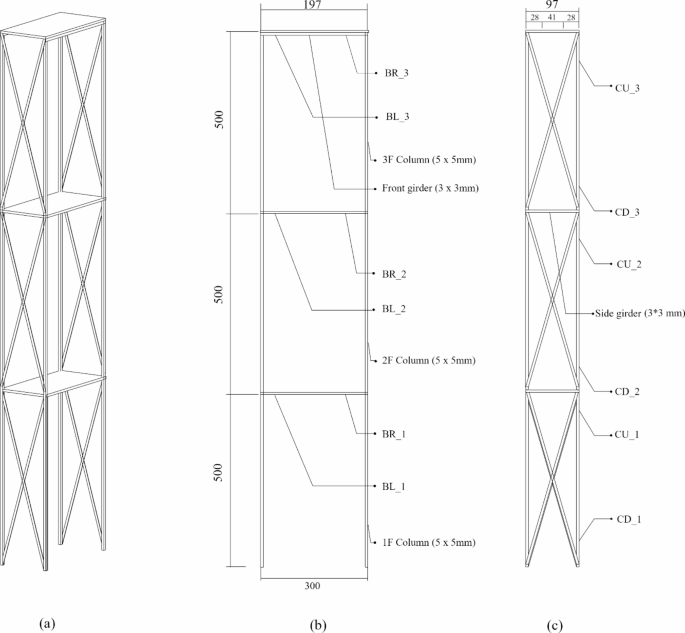
Frame structure in the numerical validation: (a) 3D view; (b) sensor installation of beams; (c) sensor installation of columns.
CWT Data generation
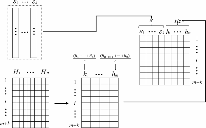
In the presented method, information on frequency data for the time-series of the structural response subjected to the seismic load is utilized in the training process of the CNN to predict the dynamic strain responses of the faulted sensor in the target structural member. To this end, the CWT results for the time-series of strain data obtained from the sensor installed on the adjacent structural member were additionally set as the input in the CNN. In generating CWT data, the effective range in the frequency domain is set and reflected in the CNN input data considering the natural frequency of the target structure to be monitored. The size of the input data and the number of frequencies used in the CWT do not match. In general, as the number of frequencies increases, the size of the CWT data increases, and the resolution of the signal processing result increases. Therefore, to adjust the size of CWT data, a method for adjusting the number of frequencies used in the CWT is presented as follows:
The method for adjusting the size of CWT data is illustrated in Fig. 5. In the method, the arithmetic mean of the CWT data is used to reduce the size of the CWT data. In the arithmetic mean calculation, a constant \(\:k\) is determined, which is the number of adjacent members used in the CNN input data. \(\:n\:\)is the number of frequencies used in the CWT, and \(\:m\:\)is the reduced number of frequencies after the reduction process of the number of frequencies. The shape of the input data in the CNN is a square form in the study. The length of one side of the square is S. Thus, the size of the input data in the CNN is S by S. The relationship given in Eq. (10) is established as below.
In addition, variables \(\:n\) and \(\:m\:\)satisfy the relationship given in Eq. (11). In Eq. (11), constants c and d are integers that satisfy the relationship between m and n.
$$\:n=m\times\:c+d\:\:\:$$
(11)
In the method, 110 frequencies determined by \(\:\beta\:\:\)and \(\:\gamma\:\) set in the Continuous wavelet transform (CWT) section were used as the CWT data. The number of strain sensors of the adjacent structural members to be used for training was 2, and the input data size was 20 × 20. Thus, the number of frequencies \(\:m\) that can be used for training was 18. Accordingly, the values of integers c and d in Eq. (11) were determined. The effective range of the frequency data for training was selected by referring to the FFT results given in Fig. 2 (a). The selected range was 1 Hz to 10 Hz considering the natural frequencies of interest for the target structure. The number of frequencies \(\:n\) used for the CWT analysis was 110. In addition, because the input data size 20 × 20 was used for training, \(\:m\:\)was determined to be 18, excluding two strain sensors of the adjacent members. Thus, the combination of c and d can be estimated using Eq. (11). In general, as the size of c increases and the size of d decreases, the resolution of the CWT result used for input data decreases; hence, the wider range of the frequency can be reflected in the CWT data. On the other hand, as the size of c increases, the range of frequency cannot be reflected in the data decreases. Thus, a trade-off relationship between the range of frequency reflected in the training datasets and the resolution of the CWT results arises. In this study, considering the trade-off relationship and the range of the target frequency of interest, c and d were set to 6 and 2, respectively, for the input data configuration. The influences of the trade-off relationship on the prediction performance of CNN will be investigated in a future study on CWT-based response prediction. In addition, as different types of data such as CWT data and strain response were set at the same time in the input of the CNN, normalization was applied to the input data. The maximum and minimum values of each component in the input were used to normalize the data to adjust input data to having a similar scale by Eq. (12).
$$\:X=\fracx-\textm\texti\textn\left\x\right\\textmax\left\x\right\-\textm\texti\textn\left\x\right\$$
(12)
where \(\:X\) and \(\:x\) denote the normalized input data and original data, respectively. The normalized input data have values between 0 and 1 through normalization and are used in the CNN training.
Arranged method of input data for CNN training.
Results of the strain prediction
The performance of the presented method for predicting the dynamic strain responses of the example structure was examined. The strain response of CU_3 in Fig. 4(c) was selected as the prediction target which can be regarded as the response of the faulted sensor and was utilized as the output data of the CNN, while the strain responses of BR_3 and BL_3 in Fig. 4(b) were chosen as the responses of the adjacent members and were utilized as the input data of the CNN. The CWT data of the strain response measured in BR_3 was additionally utilized as the input data of the CNN. For Load Cases 1 and 2, the input and output data were generated. Using the datasets, the CNNs were trained for two load cases.
For the training datasets of Load Cases 1 and 2, CNNs were trained and the convergence curves of the trainings were shown in Fig. 6(a) and (c), respectively. As shown in the figures, considerable sharp decreases in the loss functions were observed in the very beginning stages. Due to the considerable and drastic decreases in the loss function at the initial stages, the rest of the convergences of the loss functions were not clearly observed but loss functions were steadily decreased with small variations. The time required for the training for one load case was approximately two hours (technically 7065 s. for a case). The specification of the device included a 12th Gen Core i7 (2.1 GHz) and 32GB of ram. Figure 6 (b) and (d) indicate strain prediction results for Load Cases 1 and 2, respectively. The figures reveal a good agreement between reference and prediction for both two load cases. Once the CNN was trained, the prediction by new testing data was almost immediately implemented.

CNN-based prediction results for the 3rd story column strain data using beam strain data on each load case: (a) convergence curve for Load Case 1; (b) comparison of strains between reference and prediction for Load Case 1; (c) convergence curve for Load Case 2; and (d) comparison of the strains between reference and prediction for Load Case 2.
In addition, the prediction results of the dynamic strain responses were examined. Figure 7 (a) and (b) display the prediction results for the time-series of strain data of the target structural component for Load Cases 1 and 2, respectively. In Load Case 1, the root mean square error (RMSE) and mean absolute error (MAE) for dynamic response prediction were 15.4924 and 7.6042 in Training and 64.3108 and 38.7584 in Testing. In Load Case 2, RMSE and MAE were 12.0908 and 7.5272 in Training and 53.0034 and 36.4224 in Testing. The results and figures confirmed that the predicted time series data showed a fairly good agreement with the reference data.

Prediction results of the time-series data of the 3rd story column by inputting the response of the 3rd story beam data to the trained CNN: (a) subjected to the Load Case 1 and (b) subjected to the Load Case 2.
Figure 8 emphasizes the strain prediction errors of CNNs trained with CWT data and without CWT data for Load Case 1 according to the increase in the training number. The strain prediction performances were evaluated by RMSE and MAE, as depicted in Fig. 8 (a) and (b), respectively. In the figure, the variations in RMSE and MAE values for the training and test datasets are presented according to the increase in the number of iterations during the CNN training. As the number of CNN trainings increases, the RMSE and MAE values decrease. The minimum RMSE value was calculated from about 22,000 training numbers. For the training datasets, the CNN trained with CWT data shows a slightly better performance. For the test datasets, the CNN trained with CWT data shows much better prediction performance compared to the CNN trained without CWT data. The results confirmed that the reliability of the CNN training with CWT data is higher for the dynamic strain response prediction subjected to seismic loads compared to the CNN training without CWT data, and the effectiveness of using CWT data in the presented method was verified.

CNN-based prediction results for the 3rd story column strain data according to the increase of the training number: (a) RMSE and (b) MAE.
Effectiveness of CWT
The prediction performance of the dynamic strain response according to variations in the scale of the seismic load was examined. To this end, the strain response at the location of the strain sensor installed in CU_3 which is assumed to be the faulted sensor of Fig. 4(c) was selected as the prediction target. BR_3 and BL_3 of Fig. 4(b) were selected as the adjacent members used for CNN training. The CWT data of the strain response measured in BR_3 was used as additional input data for the CNN. The CNNs were trained with structural responses obtained by ground accelerations of 18 earthquakes used in Load Case 1. In this section, test datasets were generated by scaling the remaining 2 earthquakes by the values of 0.25, 0.3, 0.35, and 0.4 and used to assess the performance of the dynamic response prediction of the trained CNN.
Figure 9 highlights the RMSE and MAE of the trained CNN for the different scales of earthquakes described above. In the case of an earthquake with a relatively small scale (0.25), the prediction performances of the CNNs trained with CWT and without CWT were almost similar. The RMSE and MAE of the CNNs trained with CWT were 30.759 and 15.4924, respectively. The RMSE and MAE of the CNNs trained without CWT were 27.219 and 14.0695, respectively.

CNN-based prediction results for the 3rd story column strain data based on the scale of earthquake acceleration: (a) RMSE of training results and (b) MAE of training results.
On the other hand, according to the increase in the earthquake scaling value, the differences in RMSE and MAE between the CNNs with and without CWT data increased. The CNNs trained with CWT data showed much better prediction performances than those trained without CWT data for larger values of scale for the earthquake. Specifically, for a 0.3 scale of an earthquake, the RMSE and MAE of the CNN trained with CWT were 64.3108 and 38.7584, while those of the CNN trained without CWT were 97.612 and 59.9739, respectively. For a 0.35 scale of an earthquake, the RMSE and MAE of the CNN trained with CWT were 94.7972 and 63.7563, while those of the CNN trained without CWT were 171.355 and 142.8577, respectively. At a 0.4 scale, the RMSE and MAE of the CNN trained with CWT were 159.839 and 103.0434, while those of the CNN trained without CWT were 248.013 and 198.0642, respectively. These findings confirm that utilizing CWT in the CNN training is effective in predicting dynamic strain response for relatively larger-scale earthquakes.
Experimental validation
Descriptions of the experimental structure
To confirm the validity of the presented method in practice and the robustness of the method for a different type of structure compared to the steel frame used in the numerical study, an additional investigation was conducted by using real data measured from another structure which was an experimental reinforcement concrete (RC) specimen. For this purpose, a shaking table test was conducted on an experimental specimen to obtain the strain response of structural components subjected to seismic loads. The experimental specimen is a multi-story frame structure as shown in Fig. 10. The story height is 1.2 m, and the total height of the specimen is 3.6 m. Detailed information on the dimensions of the specimen, the size of girders and columns that constitute the specimen, reinforcement rebar, and the strain sensor installation can be found in the literature19. The strain sensors are installed on the main rebar and hoop in the column members. The strain responses of the installed sensors were measured in the shaking table test subjected to seismic loads. In the test, the earthquakes identical to Load Case 2 presented in the numerical study in the Application section were simulated.
In this experimental study, a column of the 3rd story was selected as the target structural member where the faulted sensor is assumed to be installed, and columns of the 1st and 2nd stories were selected as the adjacent structural members. The locations of sensors used in the experimental study are shown in blue boxes in Fig. 10(a) and (b). The strain responses measured from rebars in these columns were used for CNN training. For Load Case 2, strain responses were measured from the 3rd, 2nd, and 1st story columns. The strain data measured from the 3rd column, which is the target member to be monitored, was set as the output of the CNN, and those from the 1st and 2nd columns were set as the input of the CNN. Based on the results in the Application section, where the CNN using the CWT data exhibits outstanding prediction performance compared to without CWT data, the CNN with the CWT data was considered to predict strain responses in this section. Thus, both the time-series of the strain data of the 1st and 2nd columns and CWT results of strain responses of the 2nd column were used in training the CNN.

Strain prediction results for the RC frame
Using the training datasets constituted by strain data measured in the test, the CNN was trained. Figure 11(a) exhibits the convergence curve during CNN training. It shows a drastic decrease in the loss function at the initial stage of the training and stable convergence. Figure 11(b) shows the strain prediction results of the trained CNN, where a good agreement between the reference and prediction for both training and test datasets is observed. The prediction capacity of the method using the CWT data was confirmed again in this experimental study.

CNN-based prediction results for the 3rd story column strain data using the 2nd story column strain data on load case: (a) convergence curve of Load Case 2 and (b) strain prediction results of Load Case 2 training.
Figure 12(a) compares the time-series of strain responses between the reference and prediction. RMSEs of predicted strain responses are 5.6715 and 7.5199 for training and test datasets, respectively. MAEs of predicted strain responses are 4.4794 and 5.9699 for training and test datasets, respectively. It can be inferred that the strain responses were fairly well predicted in terms of time series forecasting of data, such as frequency, phase, and amplitude. Figure 12(b) reveals the prediction results of the time-series of strain data where the maximum displacement occurred. It was confirmed that predicted strain values were well matched to the observation values at the time when large responses occurred.

CNN-based prediction results of the time-series of the 3rd story column strain data by using the response of the 1st and 2nd story columns: (a) subjected to the Load Case 2 and (b) enlarged plot of Fig. 12 (a).
link